1. Introduction
This article aims to integrate the models presented, the Kuz-Ram and crushing with selective circulation. If you have not read, I make the links available:
Fragmentation of rocks using explosives: Brief concepts and Kuz-Ram model – Part II (M2M):

Unraveling the crushing model with selective circulation: Part III (M2M):

Here I will bring an optimization process with the aim of minimizing the unit cost (€/m3) that involves these two operations. For this, this part will be divided into two points for the understanding of the reader, which are:
• Choice of the crusher and optimization of the kinetic parameters that govern the selective circulation crushing model;
• Description of an optimization model for the integration of the KuzRam model with that of selective circulation crushing.
For today we will discuss only the point that is highlighted in bold.
2. Choice of crushing equipment
The machine chosen in this example to process the fragmentation of the material from the disassembly generated by the Kuz-Ram model was the Nordberg® C200 ™ jaw crusher. This crusher has some relevant characteristics that should be mentioned:
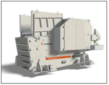
Maximum granulometry – top-size: up to 1500 mm.
• Regulation: close side setting – the minimum is 175mm, while the maximum is 300mm;
• Capacity: minimum 630 t/h and maximum 1435 t/h. These values depend directly on the regulations that will be used;
• Throw: 50mm.
As we already know the intervals that govern the close side setting and also its throw, we can find the open side setting through the following expression:
OSS = CSS + Throw
So if a 300 mm CSS is used, we will have the following OSS:
OSS = 300 + 50 = 350 mm
In this way we have an OSS and CSS of 350 mm and 300 mm respectively, values used to adjust the crushing model that will be addressed later in another article.
3. Method for adjusting the crushing model
The adjustment of the model was made in an open circuit, with a fixed feed and in a stationary regime. As already mentioned, the crushing model is governed by four kinetic parameters, being:
• Destruction matrix, Si – Pa and Pk;
• Formation Matrix, Bij – m1 and m2.
Adjustments can be made using some software, such as MATLAB or Excel. For simplicity, I used Excel using the Solver function. With this tool it is possible to find maximum or minimum values (optimized value) for a given cell formula in Excel. This same cell is called the objective function (F.O) and is subject to restrictions (S.A) and decision variables (V.D.). The strategy adopted for the recovery of kinetic parameters was:
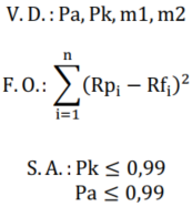
Being:
Rpi: Cumulative of the particle size distribution cataloged by Metso to a 300mm CSS, for a certain “i” class;
Rfi: Cumulative of the particle size distribution simulated by the crushing model, for a certain “i” class.
4. Optimization of kinetic parameters
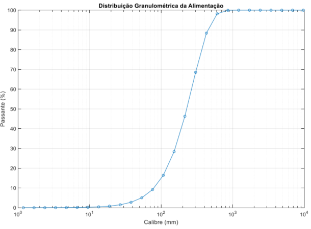
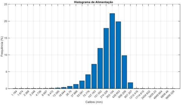
The data for the adjustment was given first from the Kuz-Ram model, generating the feed material of the crusher that will give the final product after the simulation process. The cumulative of the feed, as well as the class of histograms generated by this process can be seen below:
As in this example, I do not have a real sample of the crusher product to optimize the kinetic parameters of the crushing process, I used cataloged particle size curves for different crushing equipment from Metso (jaw crushers).
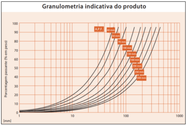
Figure 4 shows the granulometric curves (Metso, 2013) generated for different CSS’s of the equipment. In this specific case, the particle size curve corresponding to a close side setting of 300 mm was chosen in order to optimize the kinetic parameters. Each point obtained was collected from the predefined Tyler scale. The entire optimization process that I have shown here was elaborated in Excel, and followed the strategy for correction as discussed in the topic “Method for adjusting the crushing model”.
The results obtained using Solver to correct the kinetic parameters were:
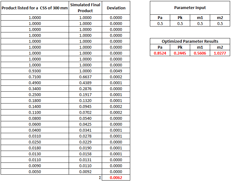
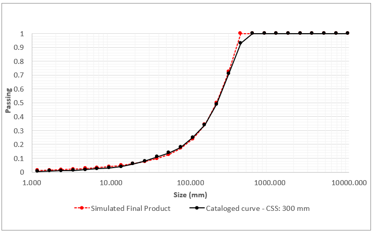
After the optimization process it can be seen that the size distribution curves generated by the simulation process, and the size distribution curve represented in the catalog for a 300 mm CSS are practically overlapping, obtaining a residue of only 0.0062.
In summary we obtained the following optimized parameters:
• Pa: 0,8524;
• Pk: 0,2445;
• m1: 0,5606;
• m2: 1,0277.
Okay, Auã. But what are these values for? What can I do with them?
Once the simulation model is calibrated, with the determination of the kinetic parameters, which describe the fragmentation operated by a jaw crusher, it will be possible to test different configurations, such as varying the feed granulometry, or varying the CSS. However, the crusher’s working conditions should be respected, and since it is equipment of defined geometric constriction, it will be necessary to maintain their reduction ratios between 4:1 and 8:1 in this case.
5. Conclusion
I hope you enjoyed. Next week I will bring more about the blast and crushing interaction process.
Stay safe 🙂