1. Introduction

At the beginning of the 1970s, the first matrix crushing models emerged, one of which was proposed by mining engineer Alban Lynch.

He was a pioneer in the use of computers for the development of fragmentation and classification models, validating his studies at the Mount Isa Mines ore treatment plant, currently belonging to the Glencore group. The model proposed by Lynch was developed for machines with fixed residence time, in which it calls for a finite transition function. The finite transition represents the change in size over a given finite time interval, equal to the average and constant residence time for all particles. In other words, this is a perfect transport flow because it allows the same residence time for all particles that are in the process.

Soon:

fi: feed composition vector;

M: mass flow through the crusher;

pi: vector composition of the final product.

The mass balance equations for each size that describe this circuit in steady state regime are given by:

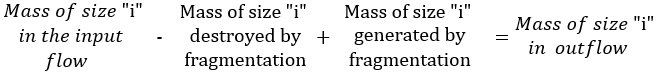
In addition to the study of fragmentation laws, the mass balance above can be described as a kinetic process by the following equation:

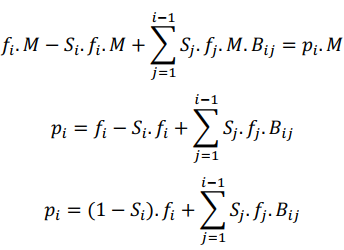
Being:

Si: size destruction function by the fragmentation process;

Bij: formation function, which corresponds to new particles formed by the fragmentation of the larger sizes that have been destroyed.

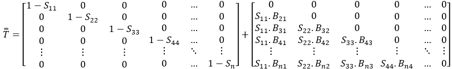
The above equation is represented by the following matrix form:

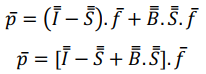
Here we can use the transition matrix, which applied to the initial composition vector returns another final composition vector:

Substituting in the previous equation we have:

It is worth noting at this point that the close side setting (CSS) and open side setting (OSS) of the fragmentation equipment are not yet expressed in the final formula of the model. Before presenting it here, it is necessary to first understand the kinetic parameters that govern the fragmentation process that was previously presented, and after that, the selective circulation matrix model proposed by Lynch will be demonstrated.

Here I will leave a short video of how a jaw crusher works:

2. Fragmentation kinetics parameters

As previously postulated by the equation that governs the matrix model of perfect transport crushing, it was seen that there is a need to determine two matrices that were presented as Si and Bij, which are named respectively by destruction and formation function.

There are four kinetic parameters that characterize the destruction and formation functions. These are called Pa, Pk, m1 and m2.

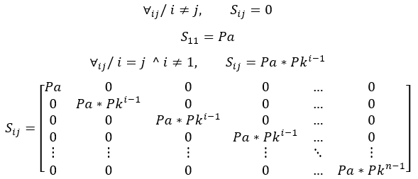
Regarding the destruction matrix, the parameters that characterize it are:

• Pa: is the measure of useful fragmentation energy, and is dependent on the energetic conditions in which the comminution process operates.
• Pk: this parameter is less than 1, it associates the characteristics of the ore with the destruction function and also commands the decrease of this.

Regarding the formation matrix, the parameters used are m1 and m2, and there is a principle in the use of Harris’ granulometric law. According to Leite (Leite, 1984) they are defined as:

m1: controls the fine particles section of the cumulative curve;

m2: controls the section of coarse particles of the cumulative curve.

The challenge will start now. Get a cup of coffee and come with me 🙂

2.1 Matrix destruction, Si

The destruction matrix is the percentage of material that is destroyed in a singular event in a given “i” batch . There is a gradual description of the phenomenon of destruction as the size classes decrease.

Assuming some restrictions, the matrix is calculated as follows:

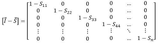
The fraction of under structured particles are shown below, with “I” being the identity matrix:

2.2 Matrix formation, Bij

The formation matrix is the way in which the products of destruction generated from a given batch are distributed to the lower (finer) sizes. In other words, it is the amount of “parent” size that will give rise to “child” sizes in the size classes worked.

The necessary parameters for the calculation of the formation matrix, are two parameters of form and one of scale. As for the shape parameters were seen previously, m1 and m2, where they adjust to the thin and large sizes respectively. While the scale parameter is represented by the maximum size generated. This same size is considered the lower limit size of the class destroyed by fragmentation.

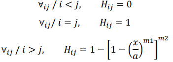
For the calculation of the formation matrix, it is necessary to use the Harris matrix. Harris’ law was chosen for the present study because it fits easily into the two sections of the normal particle size distributions as explained by Leite (Leite, 1986). This is defined based on the following restrictions:

Being:

• a: Size of the batch to be destroyed (mm);
• x: consecutive batches where the material is generated by fragmentation of “a” (mm);
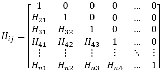
• Hij: Represents the percentage of material passing through a “x” size sieve.

Harris’ matrix takes the following form:

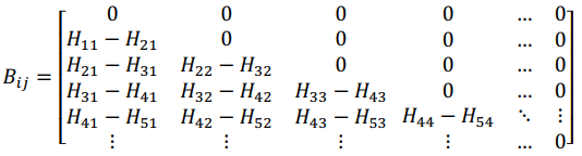
From the discretization of the data obtained from Harris, we obtain the formation matrix, Bij, represented by:

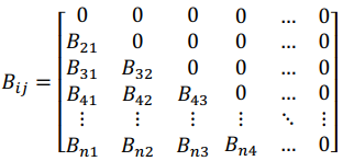
Similarly, it can be observed as:

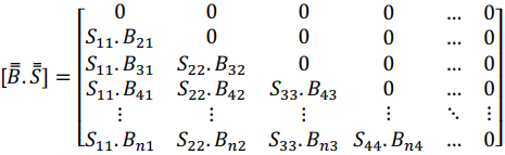
Therefore the multiplication expressed by the formation and destruction matrix, B.S, is expressed by:

2.3 Transition Matrix, T

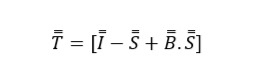
In view of what was defined as the matrix form of transition, T = [I-S + B.S], it is calculated as follows after knowing the matrices Si and Bij:

Through the sum of terms process:

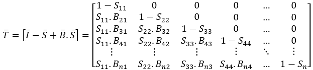
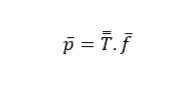
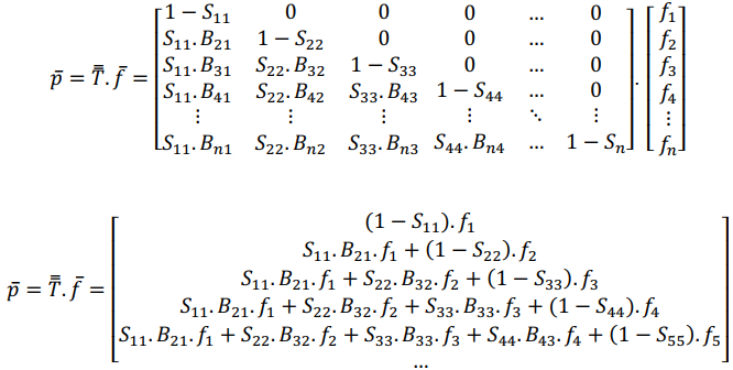
Last and not least, the final form of the crushing matrix model expressed by the perfect transport, p = T.f, takes the following form:

The article is a little long. But it is extremely important to keep this theoretical basis in mind before moving on to the final model itself. What we have just seen here is the perfect transport crushing model, that is, when all particles have the same residence time inside the crusher. But in the real world we know that this is not true.

Now you must be wondering. Okay, but where is the inclusion of CSS and OSS in the selective crushing model?

Calm down, let’s get there now.

3 Matrix model of crushing with selective circulation

In his developed model, Lynch observed that the crushing process is described by a sequence of singular events, and basically consists of a classification action and a fragmentation action. That is, during the opening of the machine any and all material is selected (contemplated by the selection function) inside the crusher chamber. The finer granulometries are discharged directly to the bottom (output) of the machine without undergoing any fragmentation process. While the larger sizes will be comminuted (designed by the transition function) and the product generated by it will be classified, being comminuted again if necessary, in a continuous manner, until the material is discharged to the equipment output.

In accordance with Futuro e Leite (Futuro e Leite, 2018) it can be concluded that the crusher’s kinetic activity is described by a finite transition that concerns the finite event, which is the comminution operation during a tightening between the jaws or cones, and by classification, which will decide which particles will be subject or not to the transition process.

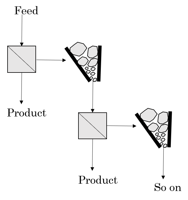
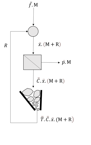
For mathematical convenience, the flow represented in figure 3 can be representative for a closed circuit, as shown in figure 4:

Being:

• M: mass flow that enters the feed;
• R: mass flow rate selected for the fragmentation event;
• f(i): histogram vector of size “i” of the feed;
• x(i): histogram vector of size “i” in the classifier feed;
• p(i): vector histogram of size “i” of the final product “;
• C(i,i): classification function, diagonal matrix that represents the probability distribution that a certain size class “i” can be fragmented;
• T(i,j): transition function, lower diagonal matrix of non-zero diagonal, representing the granulometric distribution that each granulometric fraction received after a single fragmentation event.

The balance of the flows described in figure 4 makes sense only when dealing with a closed circuit in a permanent regime. In this way, the principle of conservation of mass allows to write the mixing and classification node, where C (classification function) and T (transition function) are responsible for carrying out the transformation of the granulometric classes:

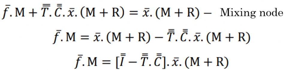
Soon:

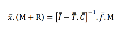
Finding it possible through this equation to determine the intermediate flow vector. Then for the classification node we have:

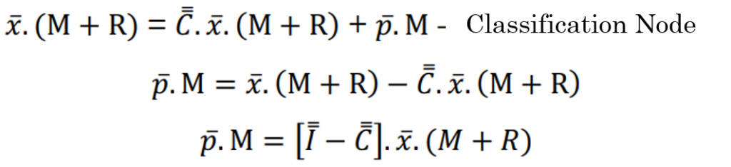
Replacing x.(M + R) with the final equation generated by the mixing node, we obtain the model proposed by Lynch for the selective circulation crushing operation, where the relationship is given by:

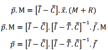
The matrix model of crushing is presented in a convenient way, since the vectors of mass inflows and outflows, defined respectively by f and p, refer to the same total flow in steady state, therefore the vectors of mass flow also constitute the histograms. of a certain size class.

4 Classification function

As already mentioned, there is a preference for fragmentation of some particles of relatively larger size compared to smaller particles. In order to understand the phenomenon of which granulometric class will undergo fragmentation inside the crushing chamber, the classification function must be used. This is represented by a probability curve that indicates the probability that a given class of size “i” will suffer a new fragmentation event, as seen in figure 5.

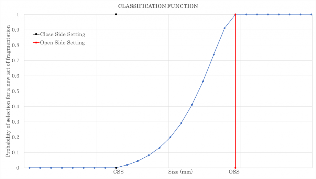
It can be seen that, particles smaller than CSS – Close Side Setting, have a probability of fragmentation equal to zero while particles larger than OSS – Open Side Setting have a 100% probability of suffering a fragmentation event. Particles of size between CSS and OSS have a probability other than zero and 100% and that can be represented by the parabolic curve. Lynch describes the classification function as a paraboloid, which can be calculated by the equations:

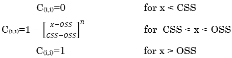
Being:

• CSS: Close side setting (mm);
• OSS: Open side setting (mm);
• x: particle size (mm);
• n: forms the function of the granulometries between CSS and OSS. The recommended value for this exponent is between 2 and 2.3.

5 Conclusion

I think I managed to make things a lot easier behind this model.

I hope you enjoyed it.

NEXT PART